Section 02 Data wrangling and quick plots
Prerequisites
Install the following packages:
tidyrdplyrggplot2
Load the libraries with R:
## Warning: 程序包'tidyr'是用R版本4.5.2 来建造的## Warning: 程序包'dplyr'是用R版本4.5.2 来建造的##
## 载入程序包:'dplyr'## The following objects are masked from 'package:stats':
##
## filter, lag## The following objects are masked from 'package:base':
##
## intersect, setdiff, setequal, union## Warning: 程序包'ggplot2'是用R版本4.5.2 来建造的Section Example: weather data from BaoAn airport
Environment data, expecially raw observations, are really messy. Here we take a look at hourly weather data measured at BaoAn International Airport during the past 10 years. The data set is from NOAA Integrated Surface Dataset.
Download the file 2281305.zip,
where the number 2281305 is the site ID.
Extract the zip file, you should see a file named
2281305.csv.
Open the file, you see many columns and even more lines, with no clear meaning and definitions. This is very often you would encounter when work with environmental data. As Hadley Wickham puts it, “Tidy datasets are all alike, but every messy dataset is messy in its own way.”
The notes below are modified from the excellent Dataframe Manipulation and freely available on the Software Carpentry website.
Loading a .csv file
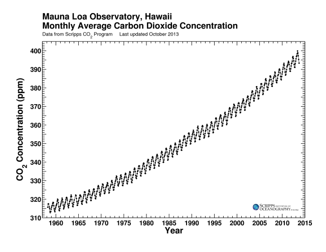
Charles David Keeling directed a program to measure the concentrations of CO2 in the atmosphere that continued without interruption from the late 1950s through the present. This program, operated out of Scripps Institution of Oceanography, is responsible for the Mauna Loa record, which is almost certainly the best-known icon illustrating the impact of humanity on the planet as a whole. Learn more about Keeling Curve Lessons.
We will start with monthly CO2 data measured from Mauna Loa.
To begin with,
Download the
co2_mm_mlo.csvfile from hereSave the file to your
working directory.Take a look at the file, where the column
co2means monthly average CO2 in the unit ofppm(part per million, 10-6),qualitycolumn is the quality flag of the observation,0means the data point does not meet the quality control so that should be discarded,1means the data point is usable.
Now let’s load this file via the following:
The file is loaded into the dataset Keeling_Data. Here
we use the option header = T so that the first
line of co2_mm_mlo.csv is also loaded as names of the
variables. You can try to turn this off by setting
header = F, and check what happens.
Check the names of columns:
## [1] "year" "month" "decimal_date" "co2" "quality"If column names are not specified, e.g., using
headers = FALSE in a read.csv() function, R
assigns default names V1, V2, …,
Vn.
Check the head (first 6 lines) of the dataset using
head() function
##   year month decimal_date    co2 quality
## 1 1958     3     1958.203 315.70       1
## 2 1958     4     1958.288 317.45       1
## 3 1958     5     1958.370 317.51       1
## 4 1958     6     1958.455 -99.99       0
## 5 1958     7     1958.537 315.86       1
## 6 1958     8     1958.622 314.93       1
Or the end of (last 6 lines) with tail():
##     year month decimal_date    co2 quality
## 810 2025     8     2025.625 425.48       1
## 811 2025     9     2025.708 424.37       1
## 812 2025    10     2025.792 424.87       1
## 813 2025    11     2025.875 426.46       1
## 814 2025    12     2025.958 427.49       1
## 815 2026     1     2026.042 428.62       1
The read.table() function is used for reading in
tabular data stored in a text file where the columns of
data are separated by punctuation characters such as .csv
files (csv = comma-separated values). Tabular files are the most common
file type you would encounter in your future study, as it’s
easy to use and share.
Tabs and commas are the most common
punctuation characters used to separate or delimit data points in
.csv files. For convenience R provides 2 other versions of
read.table(). These are: read.csv() for files
where the data are separated with commas and
read.delim() for files where the data are separated with
tabs. Of these three functions, read.csv() is
the most commonly used. If needed it is possible to override the default
delimiting punctuation marks for both read.csv() and
read.delim().
We can begin exploring our data set right away, pulling out columns
by specifying them using the $ operator:
##   [1] 315.70 317.45 317.51 -99.99 315.86 314.93 313.20 -99.99 313.33 314.67 315.58 316.48 316.65 317.72 318.29 318.15 316.54 314.80 313.84 313.33 314.81 315.58 316.43 316.98 317.58 319.03 320.04 319.59 318.18 315.90 314.17 313.83 315.00 316.19 316.89 317.70
##  [37] 318.54 319.48 320.58 319.77 318.57 316.79 314.99 315.31 316.10 317.01 317.94 318.55 319.68 320.57 321.02 320.62 319.61 317.40 316.25 315.42 316.69 317.70 318.74 319.07 319.86 321.38 322.25 321.48 319.74 317.77 316.21 315.99 317.07 318.35 319.57 -99.99
##  [73] -99.99 -99.99 322.26 321.89 320.44 318.69 316.70 316.87 317.68 318.71 319.44 320.44 320.89 322.14 322.17 321.87 321.21 318.87 317.81 317.30 318.87 319.42 320.62 321.60 322.39 323.70 324.08 323.75 322.38 320.36 318.64 318.10 319.78 321.03 322.33 322.50
## [109] 323.04 324.42 325.00 324.09 322.54 320.92 319.25 319.39 320.73 321.96 322.57 323.15 323.89 325.02 325.57 325.36 324.14 322.11 320.33 320.25 321.32 322.89 324.00 324.42 325.63 326.66 327.38 326.71 325.88 323.66 322.38 321.78 322.86 324.12 325.06 325.98
## [145] 326.93 328.13 328.08 327.67 326.34 324.69 323.10 323.06 324.01 325.13 326.17 326.68 327.17 327.79 328.93 328.57 327.36 325.43 323.36 323.56 324.80 326.01 326.77 327.63 327.75 329.72 330.07 329.09 328.04 326.32 324.84 325.20 326.50 327.55 328.55 329.56
## [181] 330.30 331.50 332.48 332.07 330.87 329.31 327.51 327.18 328.16 328.64 329.35 330.71 331.48 332.65 333.18 332.20 331.07 329.15 327.33 327.28 328.31 329.58 330.73 331.46 331.94 333.11 333.95 333.42 331.97 329.95 328.50 328.36 329.38 -99.99 331.56 332.74
## [217] 333.36 334.74 334.72 333.98 333.08 330.68 328.96 328.72 330.16 331.62 332.68 333.17 334.96 336.14 336.93 336.17 334.89 332.56 331.29 331.28 332.46 333.60 334.94 335.26 336.66 337.69 338.02 338.01 336.50 334.42 332.36 332.45 333.76 334.91 336.14 336.69
## [253] 338.27 338.82 339.24 339.26 337.54 335.72 333.97 334.24 335.32 336.81 337.90 338.34 340.07 340.93 341.45 341.36 339.45 337.67 336.25 336.14 337.30 338.29 339.29 340.55 341.63 342.60 343.04 342.54 340.82 338.48 336.95 337.05 338.58 339.91 340.93 341.76
## [289] 342.78 343.96 344.77 343.88 342.42 340.24 338.38 338.41 339.44 340.78 341.57 342.79 343.37 345.39 346.14 345.76 344.32 342.51 340.46 340.53 341.79 343.20 344.21 344.92 345.68 -99.99 347.78 347.16 345.79 343.74 341.59 341.86 343.31 345.00 345.48 346.42
## [325] 347.91 348.66 349.28 348.65 346.90 345.26 343.47 343.35 344.73 346.12 346.78 347.48 348.25 349.86 350.52 349.98 348.25 346.17 345.48 344.82 346.22 347.49 348.73 348.92 349.81 351.40 352.15 351.58 350.21 348.20 346.66 346.72 348.08 349.28 350.51 351.70
## [361] 352.50 353.67 354.35 353.88 352.80 350.49 348.97 349.37 350.42 351.62 353.07 353.43 354.08 355.72 355.95 355.44 354.05 351.84 350.09 350.33 351.55 352.91 353.86 355.10 355.75 356.38 357.38 356.39 354.89 353.06 351.38 351.69 353.14 354.41 354.93 355.82
## [397] 357.33 358.77 359.23 358.23 356.30 353.97 352.34 352.43 353.89 355.21 356.34 357.21 357.97 359.22 359.71 359.44 357.15 354.99 353.01 353.41 354.42 355.68 357.10 357.42 358.59 359.39 360.30 359.64 357.45 355.76 354.14 354.23 355.53 357.03 358.36 359.04
## [433] 360.11 361.36 361.78 360.94 359.51 357.59 355.86 356.21 357.65 359.10 360.04 361.00 361.98 363.44 363.83 363.33 361.78 359.33 358.32 358.14 359.61 360.82 362.20 363.36 364.28 364.69 365.25 365.06 363.69 361.55 359.69 359.72 361.04 362.39 363.24 364.21
## [469] 364.65 366.48 366.77 365.73 364.46 362.40 360.44 360.98 362.65 364.51 365.39 366.10 367.36 368.79 369.56 369.13 367.98 366.10 364.16 364.54 365.67 367.30 368.35 369.28 369.84 371.15 371.12 370.46 369.61 367.06 364.95 365.52 366.88 368.26 369.45 369.71
## [505] 370.75 371.98 371.75 371.87 370.02 368.27 367.15 367.18 368.53 369.83 370.76 371.69 372.63 373.55 374.03 373.40 371.68 369.78 368.34 368.61 369.94 371.42 372.70 373.37 374.30 375.19 375.93 375.69 374.16 372.03 370.92 370.73 372.43 373.98 375.07 375.82
## [541] 376.64 377.92 378.78 378.46 376.88 374.57 373.34 373.31 374.84 376.17 377.17 378.05 379.06 380.54 380.80 379.87 377.65 376.17 374.43 374.63 376.33 377.68 378.63 379.91 380.95 382.48 382.64 382.40 380.93 378.93 376.89 377.19 378.54 380.31 381.58 382.40
## [577] 382.86 384.80 385.22 384.24 382.65 380.60 379.04 379.33 380.35 382.02 383.10 384.12 384.81 386.73 386.78 386.33 384.73 382.24 381.20 381.37 382.70 384.19 385.78 386.06 386.28 387.34 388.78 387.99 386.61 384.32 383.41 383.21 384.41 385.79 387.17 387.70
## [613] 389.04 389.76 390.36 389.70 388.24 386.29 384.95 384.64 386.23 387.63 388.91 390.41 391.37 392.67 393.21 392.38 390.41 388.54 387.03 387.43 388.87 389.99 391.50 392.05 392.80 393.44 394.41 393.95 392.72 390.33 389.28 389.19 390.48 392.06 393.31 394.04
## [649] 394.59 396.38 396.93 395.91 394.56 392.59 391.32 391.27 393.20 394.57 395.78 397.03 397.66 398.64 400.02 398.81 397.51 395.39 393.72 393.90 395.36 397.03 398.04 398.27 399.91 401.51 401.96 401.43 399.27 397.18 395.54 396.16 397.40 399.08 400.18 400.55
## [685] 401.74 403.34 404.15 402.97 401.46 399.11 397.82 398.49 400.27 402.06 402.73 404.25 405.06 407.60 407.90 406.99 404.59 402.45 401.23 401.79 403.72 404.64 406.36 406.66 407.54 409.22 409.89 409.08 407.33 405.32 403.57 403.82 405.31 407.00 408.15 408.52
## [721] 409.59 410.45 411.44 410.99 408.90 407.16 405.71 406.19 408.21 409.27 411.03 411.96 412.18 413.54 414.86 414.15 411.96 410.17 408.76 408.74 410.47 411.97 413.59 414.32 414.71 416.42 417.28 416.58 414.58 412.75 411.49 411.48 413.10 414.23 415.49 416.72
## [757] 417.61 419.01 419.09 418.92 416.90 414.42 413.26 413.90 414.97 416.67 418.13 419.24 418.76 420.19 420.97 420.94 418.85 417.15 415.91 415.74 417.47 418.99 419.48 420.30 420.98 423.35 424.00 423.68 421.83 419.68 418.51 418.82 420.46 421.86 422.80 424.55
## [793] 425.38 426.51 426.90 426.91 425.55 422.99 422.03 422.38 423.85 425.40 426.65 427.09 428.15 429.64 430.51 429.61 427.87 425.48 424.37 424.87 426.46 427.49 428.62
Let’s do some simple statistical checks with
Keeling_Data$co2:
## [1] -99.99## [1] 430.51## [1] -99.99 430.51## [1] 357.1249## [1] 355.95## Min. 1st Qu. Median Mean 3rd Qu. Max.
## -99.99 330.80 355.95 357.12 386.90 430.51You will find there are some -99.99 values, which are
missing values. We will get back to this later.
You can use [] to extract elements of a vector by
specifying their corresponding index.
Important: Index
in R starts from 1, not 0. For example:
## [1] 315.70 317.45 317.51 -99.99 315.86 314.93 313.20 -99.99 313.33 314.67## [1] 1974 1974 1974 1975 1975 1975 1975 1975 1975 1975 1975## numeric(0)Tidy data
In the rest of the section, we will learn a consistent way to
organize the data in R, called tidy data. Getting the
data into this format requires some upfront work, but that work pays off
in the long term. Once you have tidy data and the tools provided by the
tidyr, dplyr and ggplot2
packages, you will spend much less time munging/wrangling data from one
representation to another, allowing you to spend more time on the
analytic questions at hand.
Tibble
For now, we will use tibble instead of R’s traditional
data.frame. Tibble is a data frame, but they tweak some
older behaviors to make life a little easier.
Let’s use Keeling_Data again:
##   year month decimal_date    co2 quality
## 1 1958     3     1958.203 315.70       1
## 2 1958     4     1958.288 317.45       1
## 3 1958     5     1958.370 317.51       1
## 4 1958     6     1958.455 -99.99       0
## 5 1958     7     1958.537 315.86       1
## 6 1958     8     1958.622 314.93       1
You can coerce a data.frame to a tibble
using the as_tibble() function:
## # A tibble: 815 × 5
##     year month decimal_date    co2 quality
##    <int> <int>        <dbl>  <dbl>   <int>
##  1  1958     3        1958.  316.        1
##  2  1958     4        1958.  317.        1
##  3  1958     5        1958.  318.        1
##  4  1958     6        1958. -100.0       0
##  5  1958     7        1959.  316.        1
##  6  1958     8        1959.  315.        1
##  7  1958     9        1959.  313.        1
##  8  1958    10        1959. -100.0       0
##  9  1958    11        1959.  313.        1
## 10  1958    12        1959.  315.        1
## # ℹ 805 more rows
Tidy dataset
There are three inter-related rules which make a dataset tidy:
- Each variable must have its own column;
- Each observation must have its own row;
- Each value must have its own cell;
These three rules are interrelated because it’s impossible to only satisfy two of the three.
That interrelationship leads to an even simpler set of practical instructions:
- Put each dataset in a tibble
- Put each variable in a column
Why ensure that your data is tidy? There are two main advantages:
There’s a general advantage to picking one consistent way of storing data. If you have a consistent data structure, it’s easier to learn the tools that work with it because they have an underlying uniformity. If you ensure that your data is tidy, you’ll spend less time fighting with the tools and more time working on your analysis.
There’s a specific advantage to placing variables in columns because it allows R’s vectorized nature to shine. That makes transforming tidy data feel particularly natural.
tidyr,dplyr, andggplot2are designed to work with tidy data.
The dplyr package
The dplyr package provides a number of very useful
functions for manipulating dataframes in a way that will reduce the
self-repetition, reduce the probability of making errors, and probably
even save you some typing. As an added bonus, you might even find the
dplyr grammar easier to read.
Here we’re going to cover commonly used functions as well as using
pipes %>% to combine them.
Using select()
Use the select() function to keep only the variables
(columns) you select.
## # A tibble: 815 × 3
##     year    co2 quality
##    <int>  <dbl>   <int>
##  1  1958  316.        1
##  2  1958  317.        1
##  3  1958  318.        1
##  4  1958 -100.0       0
##  5  1958  316.        1
##  6  1958  315.        1
##  7  1958  313.        1
##  8  1958 -100.0       0
##  9  1958  313.        1
## 10  1958  315.        1
## # ℹ 805 more rows## # A tibble: 815 × 1
## co2
## <dbl>
## 1 316.
## 2 317.
## 3 318.
## 4 -100.0
## 5 316.
## 6 315.
## 7 313.
## 8 -100.0
## 9 313.
## 10 315.
## # ℹ 805 more rowsThe pipe symbol %>%
Above we used ‘normal’ grammar, but the strengths of
dplyr and tidyr lie in combining several
functions using pipes. Since the pipes grammar is
unlike anything we’ve seen in R before, let’s repeat what we’ve done
above using pipes.
x %>% f(y) is the same as f(x, y)
## # A tibble: 815 × 3
##     year    co2 quality
##    <int>  <dbl>   <int>
##  1  1958  316.        1
##  2  1958  317.        1
##  3  1958  318.        1
##  4  1958 -100.0       0
##  5  1958  316.        1
##  6  1958  315.        1
##  7  1958  313.        1
##  8  1958 -100.0       0
##  9  1958  313.        1
## 10  1958  315.        1
## # ℹ 805 more rows
The above lines mean we first call the Keeling_Data_tbl
tibble and pass it on, using the pipe symbol
%>%, to the next step, which is the
select() function. In this case, we don’t specify which
data object we use in the select()
function since in gets that from the previous pipe. The
select() function then takes what it gets from the pipe, in
this case the Keeling_Data_tbl tibble, as its first
argument. By using pipe, we can take output of the previous
step as input for the next one, so that we can avoid defining and
calling unnecessary temporary variables. You will start to see the power
of pipe later.
Using filter()
Use filter() to get values (rows):
## # A tibble: 12 × 5
##     year month decimal_date   co2 quality
##    <int> <int>        <dbl> <dbl>   <int>
##  1  2000     1        2000.  369.       1
##  2  2000     2        2000.  370.       1
##  3  2000     3        2000.  371.       1
##  4  2000     4        2000.  372.       1
##  5  2000     5        2000.  372.       1
##  6  2000     6        2000.  372.       1
##  7  2000     7        2001.  370.       1
##  8  2000     8        2001.  368.       1
##  9  2000     9        2001.  367.       1
## 10  2000    10        2001.  367.       1
## 11  2000    11        2001.  369.       1
## 12  2000    12        2001.  370.       1
If we now want to move forward with the above tibble, but only with
quality == 1 , we can combine select() and
filter() functions:
## # A tibble: 808 × 3
##     year   co2 quality
##    <int> <dbl>   <int>
##  1  1958  316.       1
##  2  1958  317.       1
##  3  1958  318.       1
##  4  1958  316.       1
##  5  1958  315.       1
##  6  1958  313.       1
##  7  1958  313.       1
##  8  1958  315.       1
##  9  1959  316.       1
## 10  1959  316.       1
## # ℹ 798 more rows
You see here we have used the pipe twice, and the scripts become really clean and easy to follow.
Using group_by() and summarize()
Now try to group monthly data using the group_by()
function, notice how the output tibble changes:
Keeling_Data_tbl %>%
  dplyr::select(year, month, co2, quality) %>%
  filter(quality == 1) %>%
  group_by(month)
## # A tibble: 808 × 4
## # Groups: month [12]
## year month co2 quality
## <int> <int> <dbl> <int>
## 1 1958 3 316. 1
## 2 1958 4 317. 1
## 3 1958 5 318. 1
## 4 1958 7 316. 1
## 5 1958 8 315. 1
## 6 1958 9 313. 1
## 7 1958 11 313. 1
## 8 1958 12 315. 1
## 9 1959 1 316. 1
## 10 1959 2 316. 1
## # ℹ 798 more rowsThe group_by() function is much more exciting in
conjunction with the summarize() function. This will allow
us to create new variable(s) by using functions that repeat for each of
the continent-specific data frames. That is to say, using the
group_by() function, we split our original
dataframe into multiple pieces, then we can run functions
(e.g., mean() or sd()) within
summarize().
Keeling_Data_tbl %>%
  dplyr::select(year, month, co2, quality) %>%
  filter(quality == 1) %>%
  group_by(month) %>%
  summarize(monthly_mean = mean(co2))
## # A tibble: 12 × 2
## month monthly_mean
## <int> <dbl>
## 1 1 362.
## 2 2 362.
## 3 3 362.
## 4 4 364.
## 5 5 363.
## 6 6 364.
## 7 7 361.
## 8 8 359.
## 9 9 358.
## 10 10 358.
## 11 11 359.
## 12 12 361.Here we create a new variable (column) monthly_mean, and
append it to the groups (month in this case). Now, we get a
so-called monthly climatology.
You can also use arrange() and desc() to
sort the data:
Keeling_Data_tbl %>%
  dplyr::select(year, month, co2, quality) %>%
  filter(quality == 1) %>%
  group_by(month) %>%
  summarize(monthly_mean = mean(co2)) %>%
  arrange(monthly_mean)
## # A tibble: 12 × 2
## month monthly_mean
## <int> <dbl>
## 1 9 358.
## 2 10 358.
## 3 11 359.
## 4 8 359.
## 5 12 361.
## 6 7 361.
## 7 1 362.
## 8 2 362.
## 9 3 362.
## 10 5 363.
## 11 6 364.
## 12 4 364.Keeling_Data_tbl %>%
dplyr::select(year, month, co2, quality) %>%
filter(quality == 1) %>%
group_by(month) %>%
summarize(monthly_mean = mean(co2)) %>%
arrange(desc(monthly_mean))## # A tibble: 12 × 2
## month monthly_mean
## <int> <dbl>
## 1 4 364.
## 2 6 364.
## 3 5 363.
## 4 3 362.
## 5 2 362.
## 6 1 362.
## 7 7 361.
## 8 12 361.
## 9 8 359.
## 10 11 359.
## 11 10 358.
## 12 9 358.Let’s add more statistics to the monthly climatology:
Keeling_Data_tbl %>%
  dplyr::select(year, month, co2, quality) %>%
  filter(quality == 1) %>%
  group_by(month) %>%
  summarize(monthly_mean = mean(co2), monthly_sd = sd(co2),
            monthly_min = min(co2), monthly_max = max(co2),
            monthly_se = sd(co2)/sqrt(n()))
## # A tibble: 12 × 6
## month monthly_mean monthly_sd monthly_min monthly_max monthly_se
## <int> <dbl> <dbl> <dbl> <dbl> <dbl>
## 1 1 362. 33.6 316. 429. 4.07
## 2 2 362. 32.7 316. 427. 4.02
## 3 3 362. 32.9 316. 428. 4.02
## 4 4 364. 33.2 317. 430. 4.09
## 5 5 363. 33.2 318. 431. 4.03
## 6 6 364. 32.9 318. 430. 4.02
## 7 7 361. 33.0 316. 428. 4.00
## 8 8 359. 32.9 315. 425. 3.99
## 9 9 358. 33.0 313. 424. 4.00
## 10 10 358. 33.0 313. 425. 4.03
## 11 11 359. 33.3 313. 426. 4.04
## 12 12 361. 33.5 315. 427. 4.09Here we call the n() to get the size of a vector.
Using mutate()
We can also create new variables (columns) using the
mutate() function. Here we create a new column
co2_ppb by simply scaling co2 by a factor of
1000.
## # A tibble: 815 × 6
##     year month decimal_date    co2 quality co2_ppb
##    <int> <int>        <dbl>  <dbl>   <int>   <dbl>
##  1  1958     3        1958.  316.        1  315700
##  2  1958     4        1958.  317.        1  317450
##  3  1958     5        1958.  318.        1  317510
##  4  1958     6        1958. -100.0       0  -99990
##  5  1958     7        1959.  316.        1  315860
##  6  1958     8        1959.  315.        1  314930
##  7  1958     9        1959.  313.        1  313200
##  8  1958    10        1959. -100.0       0  -99990
##  9  1958    11        1959.  313.        1  313330
## 10  1958    12        1959.  315.        1  314670
## # ℹ 805 more rows
When creating new variables, we can hook this with a logical
condition. A simple combination of mutate() and
ifelse() facilitates filtering right where it is needed: in
the moment of creating something new. This easy-to-read statement is a
fast and powerful way of discarding certain data or for updating values
depending on this given condition.
Let’s create a new variable co2_new, it is equal to
co2 when quality==1, otherwise it’s
NA:
## # A tibble: 815 × 7
##     year month decimal_date    co2 quality co2_ppb co2_new
##    <int> <int>        <dbl>  <dbl>   <int>   <dbl>   <dbl>
##  1  1958     3        1958.  316.        1  315700    316.
##  2  1958     4        1958.  317.        1  317450    317.
##  3  1958     5        1958.  318.        1  317510    318.
##  4  1958     6        1958. -100.0       0  -99990     NA
##  5  1958     7        1959.  316.        1  315860    316.
##  6  1958     8        1959.  315.        1  314930    315.
##  7  1958     9        1959.  313.        1  313200    313.
##  8  1958    10        1959. -100.0       0  -99990     NA
##  9  1958    11        1959.  313.        1  313330    313.
## 10  1958    12        1959.  315.        1  314670    315.
## # ℹ 805 more rows
Combining dplyr and ggplot2
Just as we used %>% to pipe data along a chain of
dplyr functions we can use it to pass data to
ggplot(). Because %>% replaces the
first argument in a function we don’t need to specify the
data = argument in the ggplot() function.
By combining dplyr and ggplot2 functions,
we can make figures without creating any new variables or modifying the
data.
Keeling_Data_tbl %>%
  mutate(co2_new = ifelse(quality==1, co2, NA)) %>%
  # Make the plot
  ggplot(aes(x=decimal_date, y=co2_new)) +
  geom_line()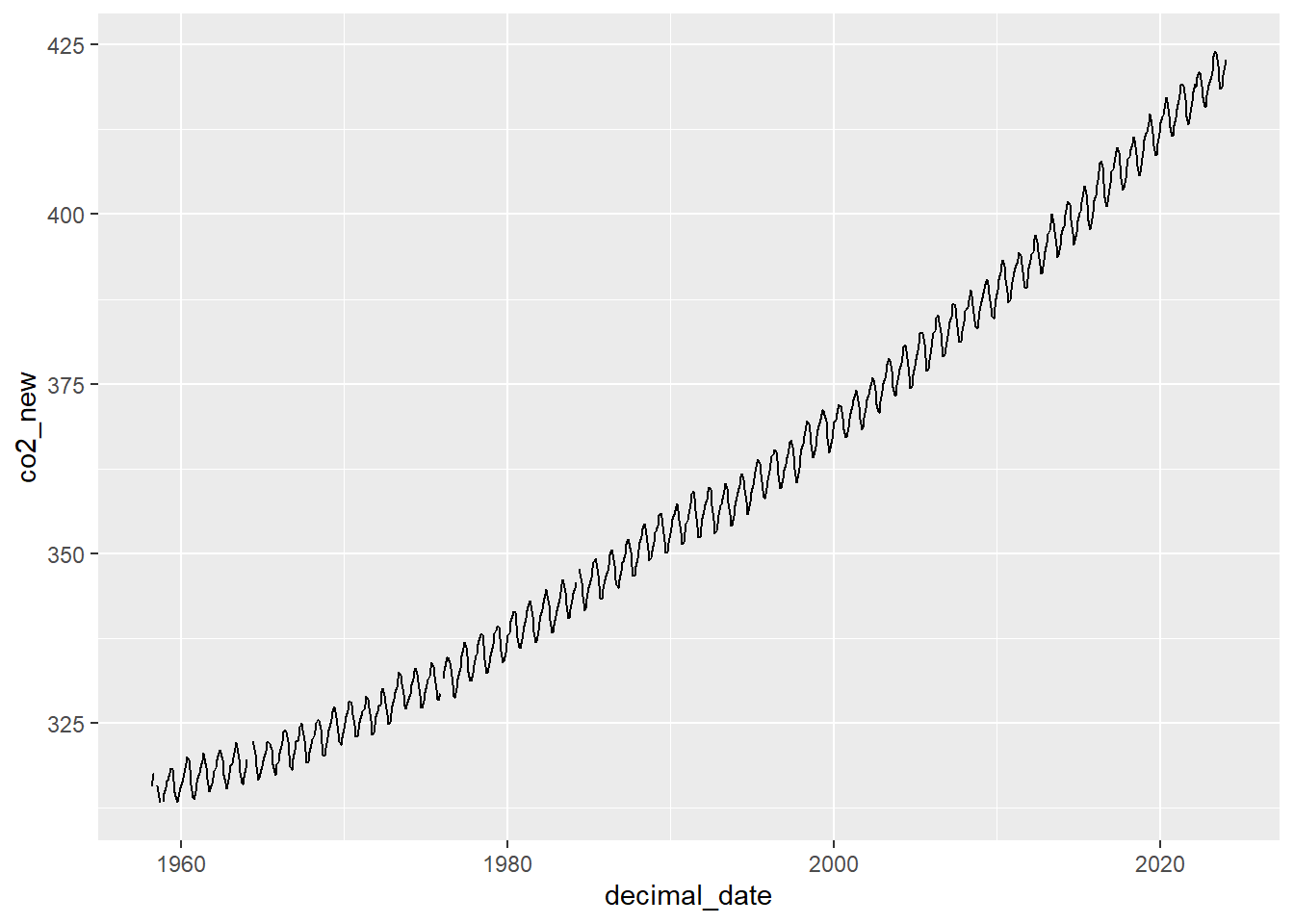
Let’s plot CO2 of the same month as a function of
decimal_date, with the color option:
Keeling_Data_tbl %>%
  mutate(co2_new = ifelse(quality==1, co2, NA)) %>%
  # Make the plot
  ggplot(aes(x=decimal_date, y=co2_new, color=month)) +
  geom_line()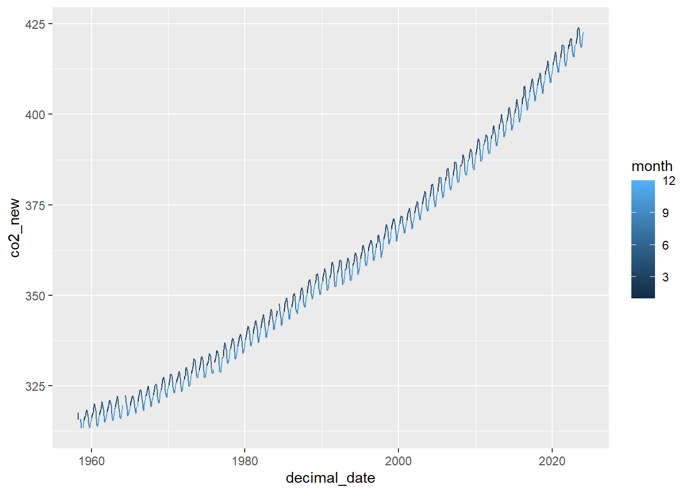
Or plot the same data but in panels (facets), with the
facet_wrap function:
Keeling_Data_tbl %>%
  mutate(co2_new = ifelse(quality==1, co2, NA)) %>%
  # Make the plot
  ggplot(aes(x=decimal_date, y=co2_new, color=month)) +
  geom_line() +
  facet_wrap(~ month)
## Warning: Removed 2 rows containing missing values or values outside the scale range (`geom_line()`).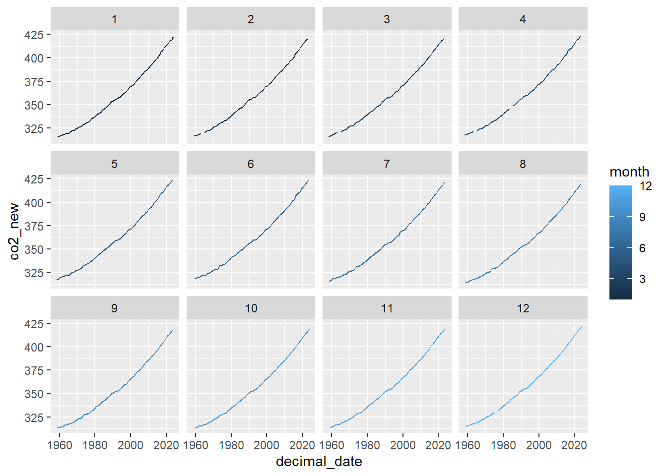
OK, that is enough for data wrangling We will learn more about
ggplot2 in future sections.
Quick plots
Now think about what will you do when get a new dataset before analyzing it?
Normally, we would like to do two things - to take a quick look at the statics and to plot the patterns.
R has many built-in functions for a large number of summary
statistics. For example, mean(), median(),
range(), max(), min(),
sd(), var(), IQR(), and
summary(). Make sure you understand how to use them and
always pay attentions to NA values.
Our next task is to visualize the data. Often, a proper visualization can illuminate features of the data that can inform further analysis. We will learn three basic types of plots in this section.
Histograms
When visualizing a single numerical variable, a histogram will be our
go-to tool, which can be created in R using the hist()
function.
# Add a new column to the original tibble
Keeling_Data_tbl <- Keeling_Data_tbl %>%
    mutate(co2_new = ifelse(quality==1, co2, NA))

# Notice we use pull() to get a vector from a tibble
Month_CO2 <- Keeling_Data_tbl %>%
  pull(co2_new)

# plot hist
hist(Month_CO2)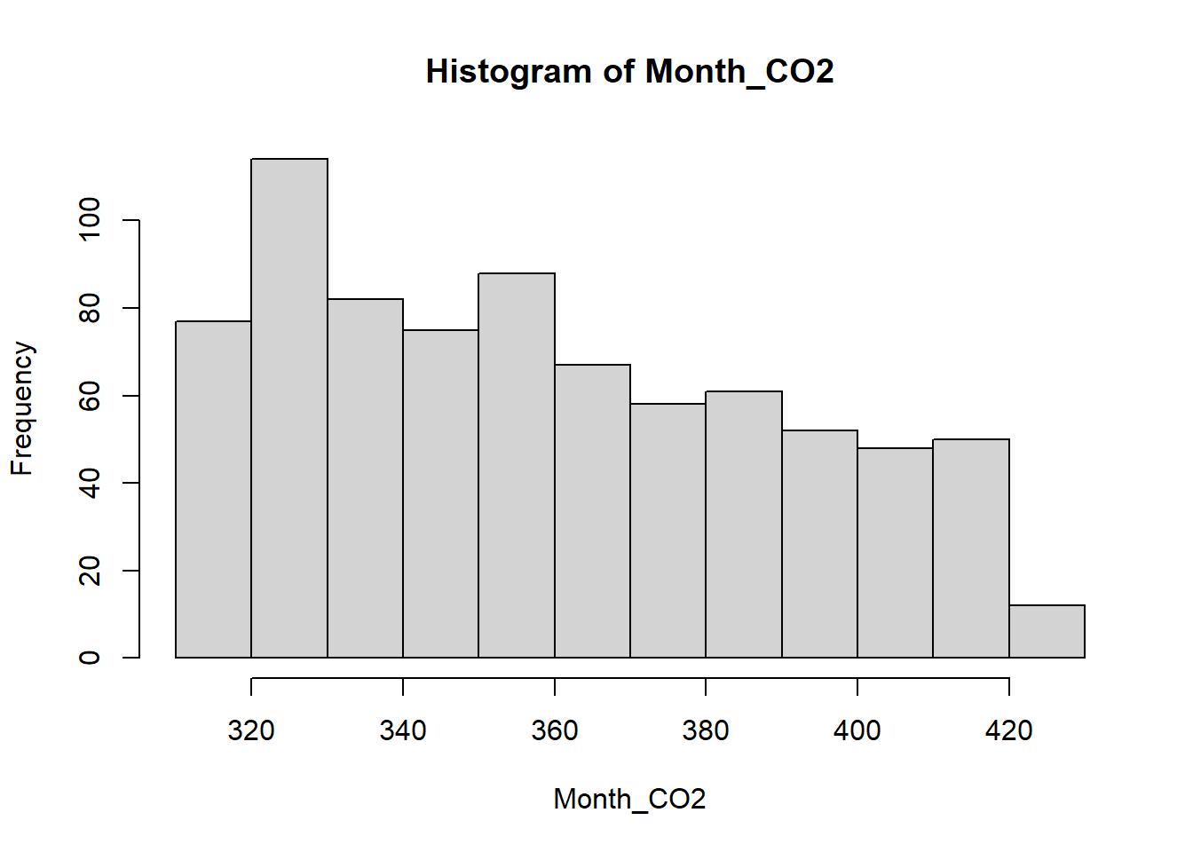
The histogram function has a number of parameters which can be
changed to make our plot look much nicer. Use the ?
operator to read the documentation for the hist() to see a
full list of these parameters.
hist(Month_CO2,
     xlab = "Monthly CO2 mixing ratios (ppm)",
     main = "Histogram of Monthly CO2",
     breaks = 20,
     col = "blue",
     border = "red")
box(lwd=2,col="green")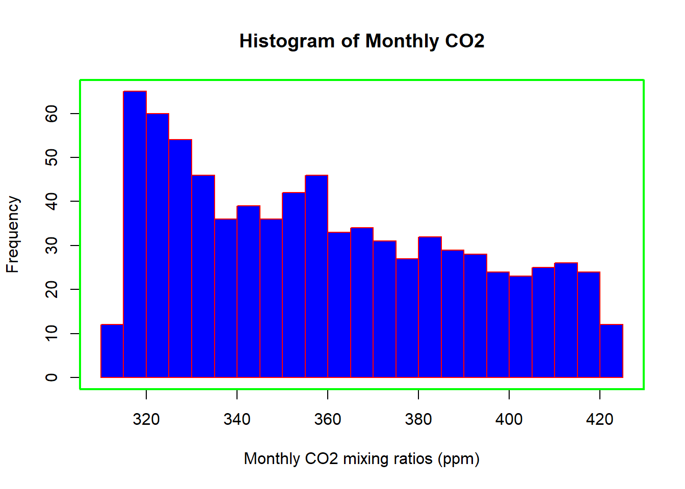
By default R will attempt to intelligently guess a good number of
breaks, but as we can see here, it is sometimes useful to
modify this yourself.
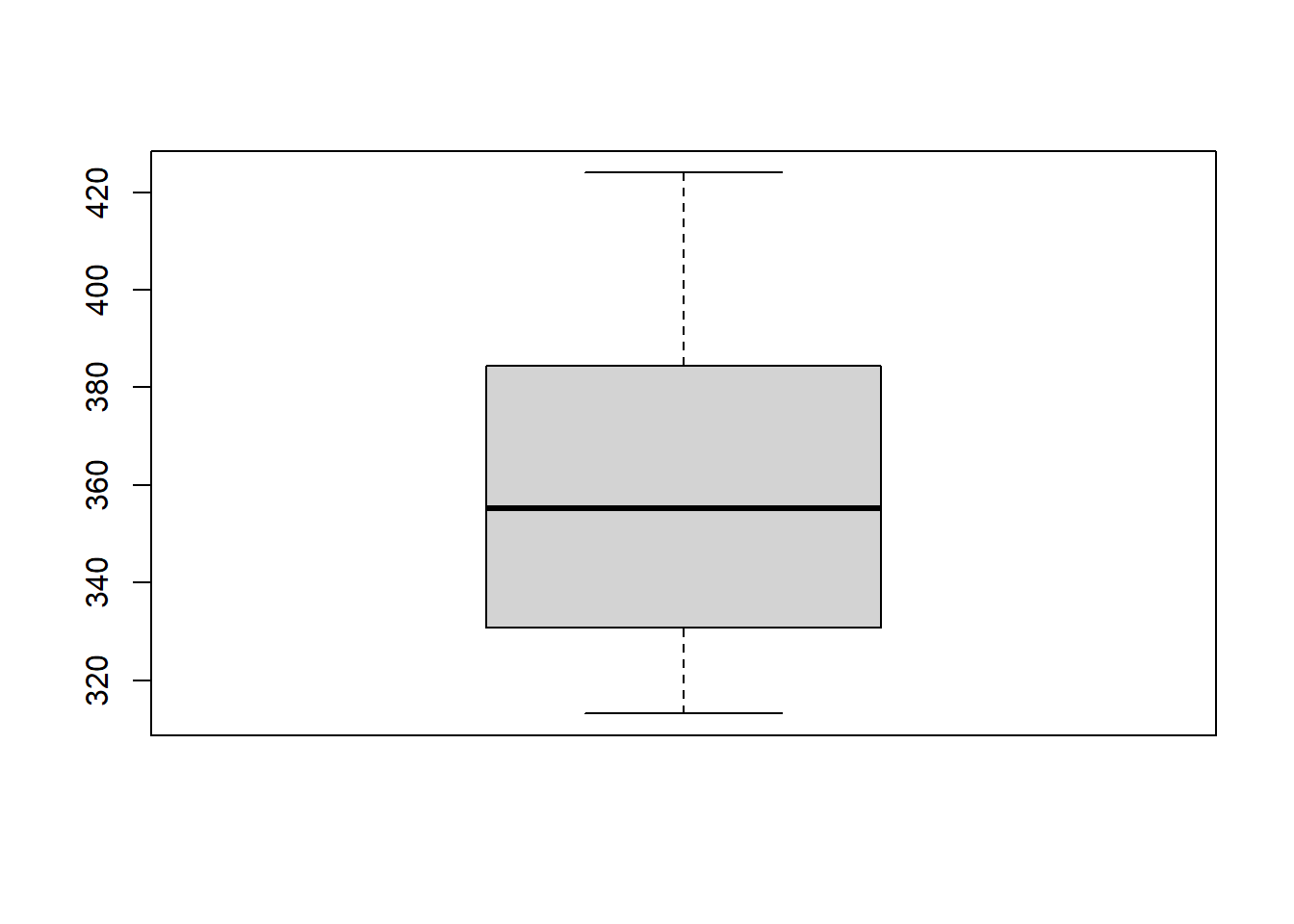
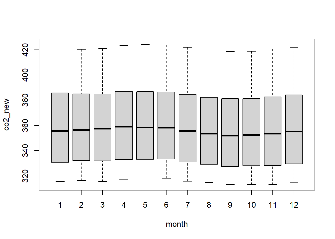
Boxplots
To visualize the relationship between a numerical and categorical
variable, we will use a boxplot. A boxplot is usful in
checking the center, spread, and skewness of a sample.
In the Keeling_Data_tbl dataset, the month
is a categorical variable. First, note that we can use a single boxplot
as an alternative to a histogram for visualizing a single numerical
variable. To do so in R, we use the boxplot() function.
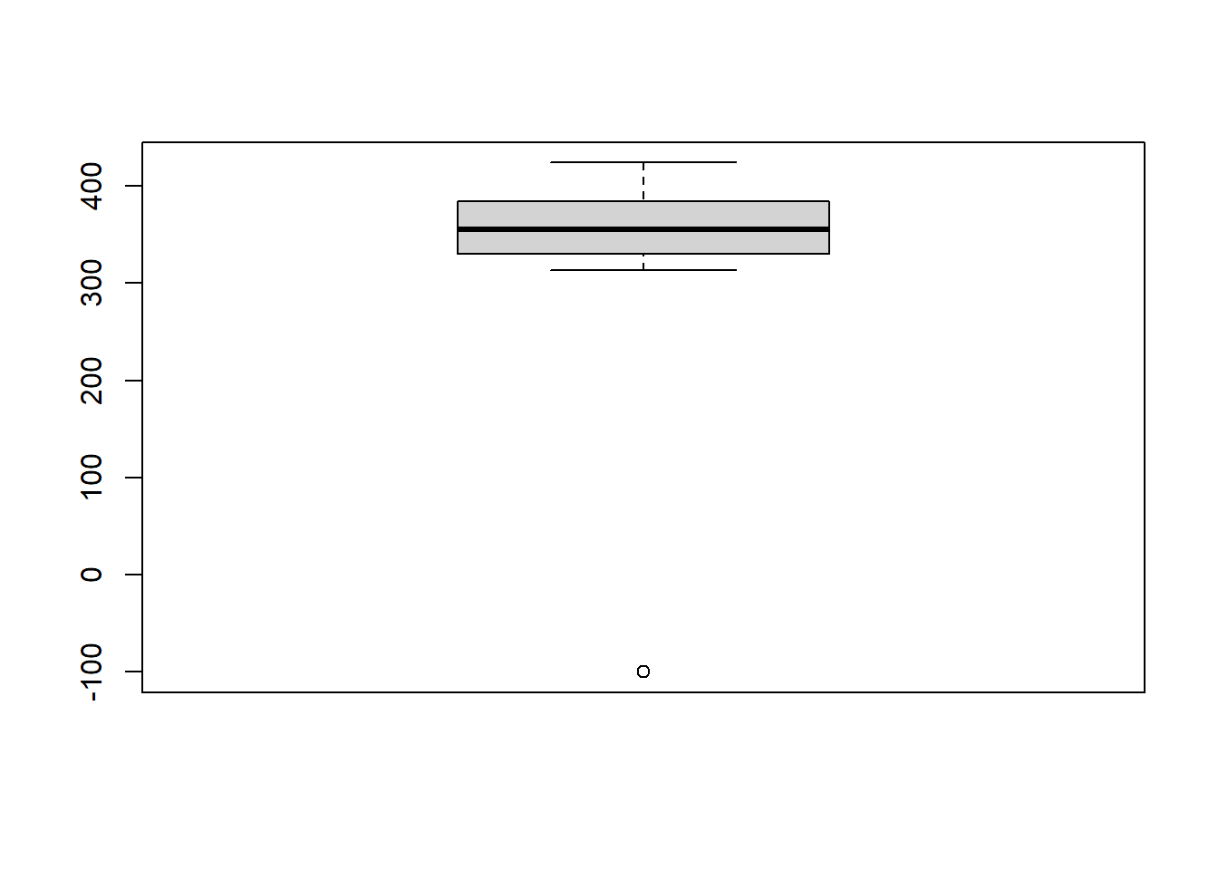
Or try to plot the raw data:
However, more often, we will use boxplots to compare a numerical variable for different values of a categorical variable.
Here we used the boxplot() command to create
side-by-side boxplots. However, since we are now dealing with two
variables, the syntax has changed. The R syntax
co2_new ~ month, data = Keeling_Data_tbl reads “Plot the
co2_new variable against the month variable
using the Keeling_Data_tbl dataset.” We see the use of a
~ (which specifies a formula) and also a
data = argument. This will be a syntax that is common to
many functions we will use later.
Again, boxplot() has a number of additional arguments
which have the ability to make our plot more visually appealing.
boxplot(co2_new ~ month, data=Keeling_Data_tbl,
xlab = "Month",
ylab = "CO2 (ppm)",
main = "Monthly CO2",
cex = 2,
col = "orange",
border = "darkgreen")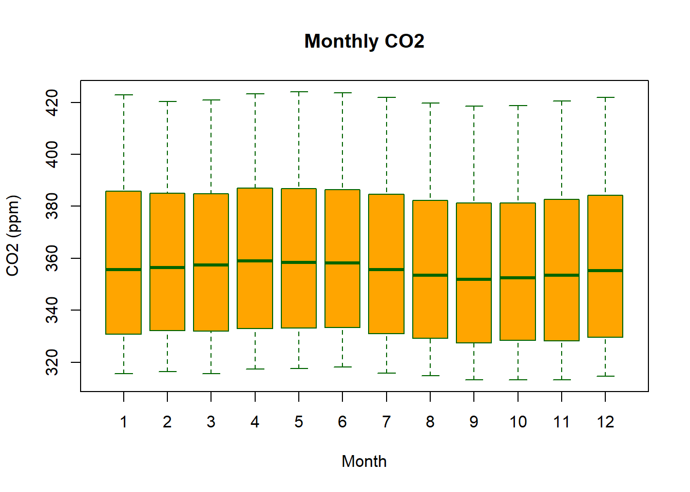
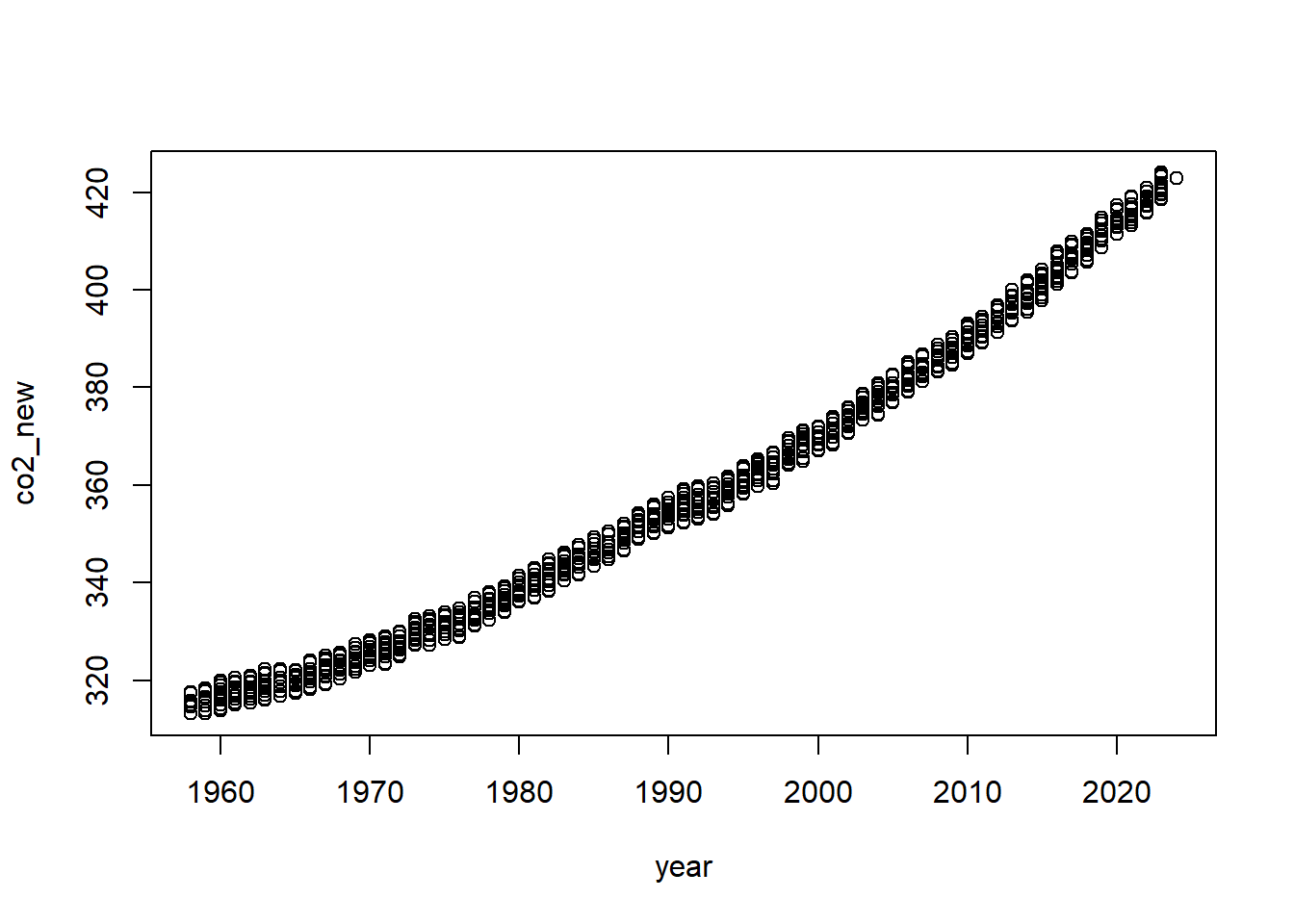
Scatterplots
Lastly, to visualize the relationship between two numeric variables,
we will use a scatterplot. This can be done with the plot()
function and the ~ syntax we just used with a boxplot. (The
function plot() can also be used more generally; see the
documentation for details.)
plot(co2_new ~ year, data=Keeling_Data_tbl,
xlab = "Year",
ylab = "CO2 (ppm)",
main = "CO2 vs Year",
pch = "+",
cex = 2,
col = "navy")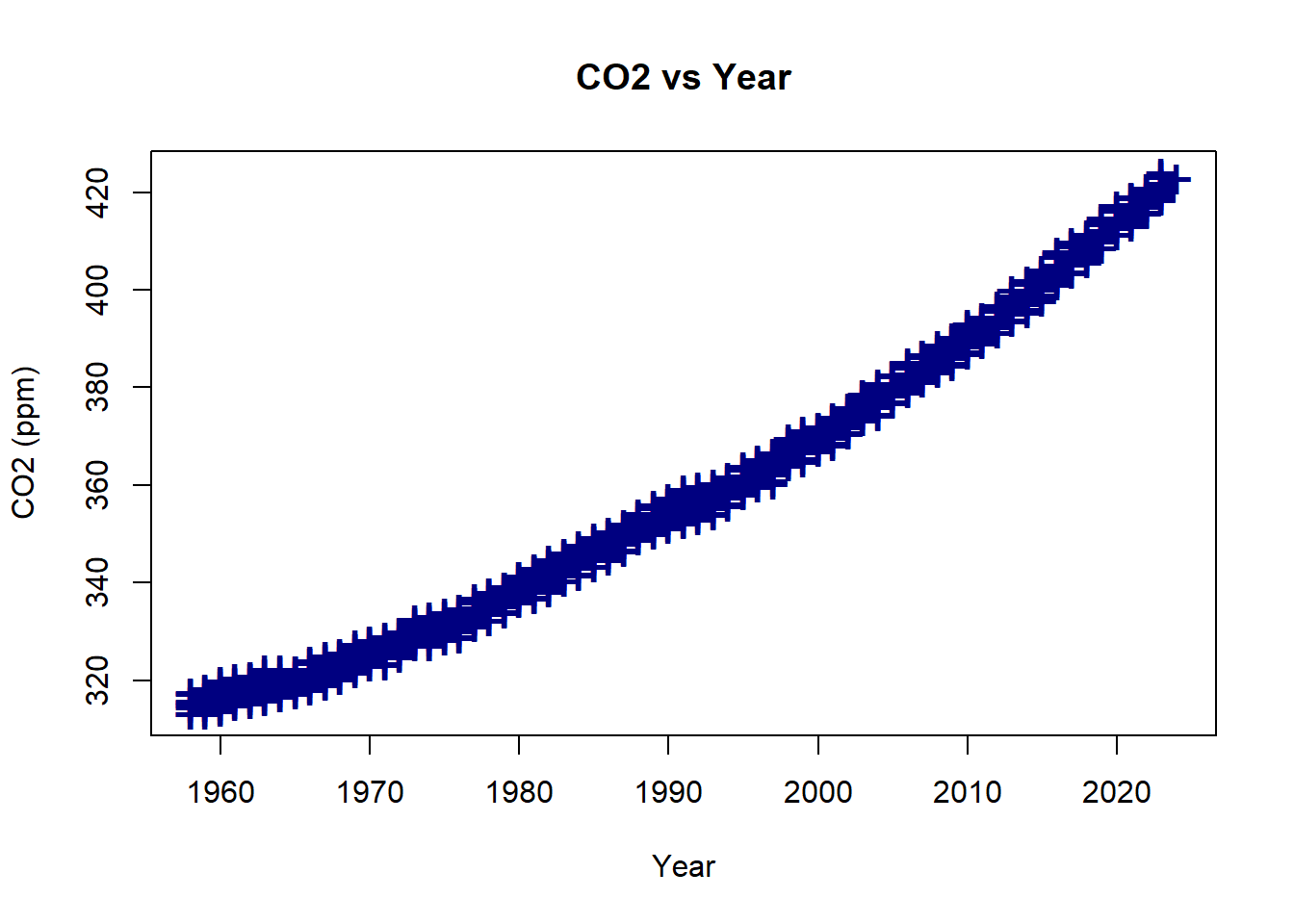
In-class exercises
Exercise #1
Use Keeling_Data, compute the annual mean of
CO2 since 1959, plot your results.
Further reading
- Data Wrangling with dplyr and tidyr Cheat Sheet
- Dataframe Manipulation with dplyr
- Dataframe Manipulation with tidyr
- R for Data Science, see chapter 10 and 12.
- Data wrangling with R, with a video