Section 07 Two-sample Z-test and t-test
Section Example: PM2.5 in Shenzhen and Guangzhou
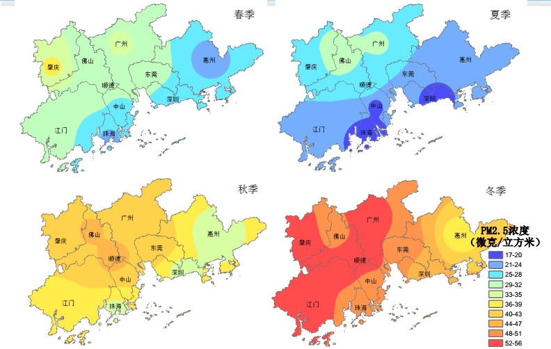
Suppose we want to compare PM2.5 levels in Shenzhen and Guangzhou. To do so, PM2.5 concentrations are measured by two groups with the same instrument.
In 2020, 10 observations are made in Shenzhen:
25.6, 23.7, 21.9, 26.0, 24.5, 22.4, 26.7, 24.6, 22.7, 23.8
and 12 observations are made in Guangzhou:
27.1, 24.2, 27.9, 33.3, 26.4, 28.7, 25.6, 23.2, 24.0, 27.1, 26.2, 24.4
We know from previous data that PM2.5 levels in the two cities
generally follow normal distributions. And the standard deviation for
Shenzhen and Guangzhou is 2.0 ug/m3 and
3.0 ug/m3, respectively.
It seems Shenzhen has a lower PM2.5 level than Guangzhou. Can such a difference be explained on the basis of chance variation? Can you explain why the spread of the data also contributes to the difference?
The Z-test
Recall the definition of Z-Ratio:
\[Z=\frac {Estimate - Parameter} {SD(Estimate)} \]
Since the task is to compare PM2.5 in the two cities, in the statistical framework, it would be:
H0: Mean PM2.5 level in Shenzhen is the same as that in Guangzhou (\(\mu_1 = \mu_2\))
H1: Mean PM2.5 level in Shenzhen is not the same as that in Guangzhou (\(\mu_1 \ne \mu_2\))
To test the hypothesis (H0), we will use Z-Ratio again. In this case, \(Estimate\) is the difference between sample averages (\(\overline{X_1} -\overline{X_2}\)), and \(Parameter\) is the difference between population mean (\(\mu_1 - \mu_2\)).
\[Z=\frac { (\overline{X_1} - \overline{X_2} ) - (\mu_1 - \mu_2) } {SD(\overline{X_1} - \overline{X_2}) } \] If the two samples are from two normal distributions, \(SD(\overline{X1} - \overline{X_2})\) can be determined as:
\[ SD(\overline{X_1} - \overline{X_2}) = \sqrt { \frac{\sigma_1^2} {n_1} + \frac{\sigma_2^2} {n_2} } \] where \(\sigma_1\) and \(\sigma_2\) is the standard deviation of the two populations, and \(n_1\) and \(n_2\) is the size of the two samples. Now we have:
\[Z=\frac { (\overline{X_1} - \overline{X_2} ) - (\mu_1 - \mu_2) } {\sqrt { \frac{\sigma_1^2} {n_1} + \frac{\sigma_2^2} {n_2} } } \] and \(Z \sim N(0,1)\).
Assuming H0 is true, we get \(Z\) is
-2.16. Then with R, we can compute the two-side p-value for
this statistic.
Before computing \(Z\), let’s check the data first.
# Shenzhen sample
SZ_PM2.5  <- c(25.6, 23.7, 21.9, 26.0, 24.5, 22.4, 26.7, 24.6, 22.7, 23.8)
SZ_n      <- length(SZ_PM2.5)
# Shenzhen population sigma
SZ_sigma  <- 2.0

# Guangzhou sample
GZ_PM2.5  <- c(27.1, 24.2, 27.9, 33.3, 26.4, 28.7, 25.6, 23.2, 24.0, 27.1, 26.2, 24.4)
GZ_n      <- length(GZ_PM2.5)
# Guangzhou population sigma
GZ_sigma  <- 3.0

# Make data frame, create a data table
PM2.5_data <- data.frame(PM2.5 = c(SZ_PM2.5, GZ_PM2.5),
                         City = c(rep("Shenzhen",SZ_n),rep("Guangzhou",GZ_n)))

# Compare boxplots
# %>% means pipe
PM2.5_data %>%
  ggplot(aes(x=as.character(City), y=PM2.5)) +
  geom_boxplot(fill="steelblue") +
  labs(title="PM2.5 Distribution by City", x="City", y="ug/m3")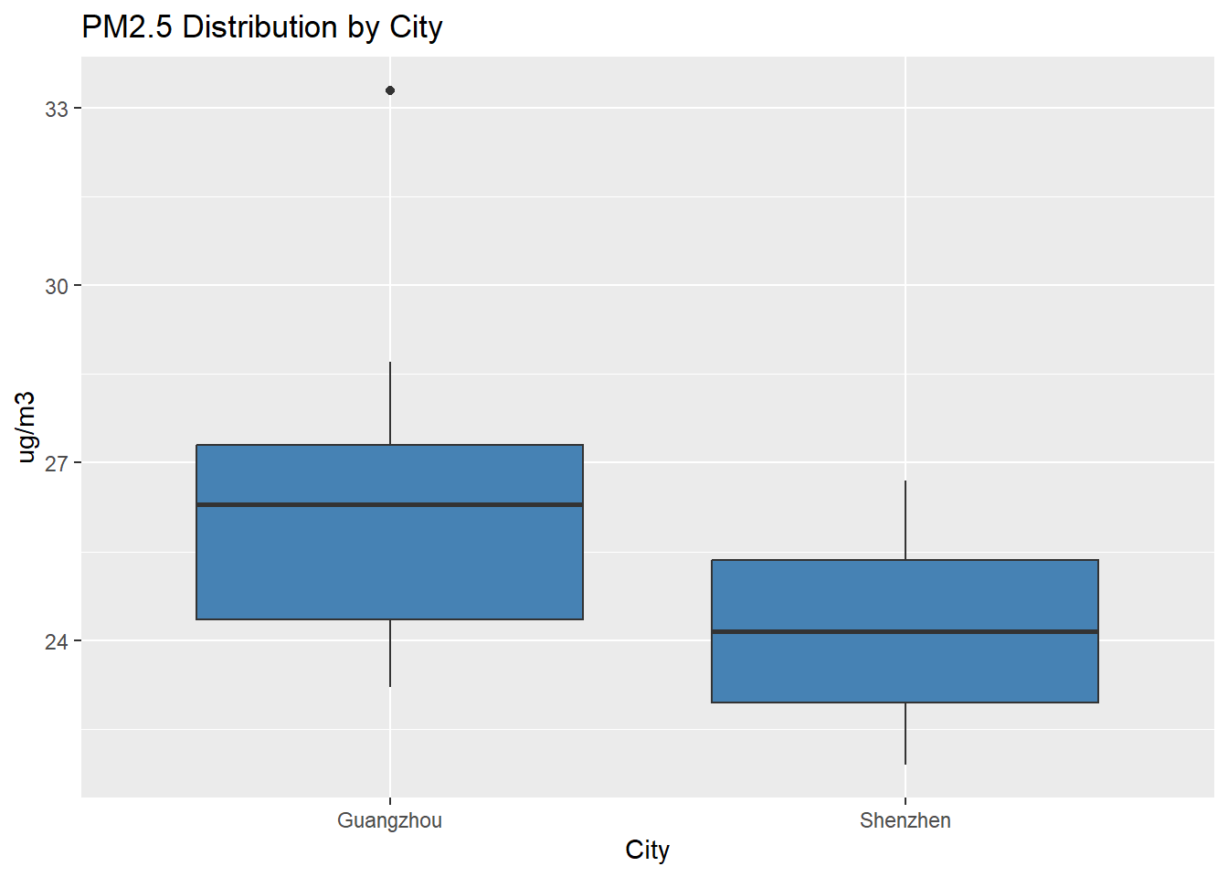
# Check normality - qqplot
PM2.5_data %>%
 ggplot(aes(sample = PM2.5)) +
  geom_qq_line() + geom_qq() +
  facet_wrap(~ City)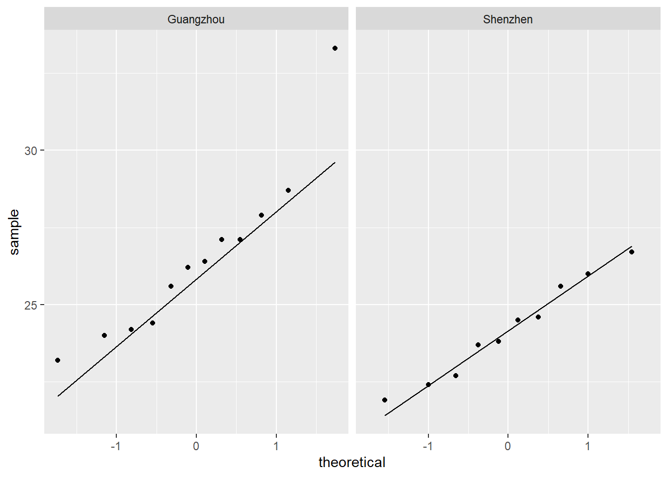
##
##  Shapiro-Wilk normality test
##
## data:  SZ_PM2.5
## W = 0.9644, p-value = 0.8346##
## Shapiro-Wilk normality test
##
## data: GZ_PM2.5
## W = 0.89343, p-value = 0.1305## [1] -2.318333# Get Z-ratio
Z <- (mean(SZ_PM2.5) - mean(GZ_PM2.5)) /
sqrt( SZ_sigma^2/SZ_n + GZ_sigma^2/GZ_n )
# Find the two-side p-value
# The pnorm function gives the Cumulative Distribution Function (CDF)
# of the Normal distribution in R, which is the probability that
# the variable takes a value lower or equal to a threshold (here |Z|).
P_value <- (1-pnorm(abs(Z), mean=0, sd=1))*2
print(P_value)## [1] 0.0306292OK, we have a probability of about 3.06% getting a
statistic (\(Z\)) as extreme or more
extreme than the observed statistic (-2.16), assuming H0 is
true. This is a small probability, and is likely due to chance. We can
reject H0 given the observations. Thus, the mean PM2.5 level in Shenzhen
is NOT the same as that in Guangzhou.
Independent two-sample t-test
As we saw from the last Section, SDs of populations (\(\sigma_1\) and \(\sigma_2\)) are generally unknown. In this case, we need to use sample SE as an estimate of the population SD, and the the proceeding Z test becomes the t test:
\[ t =\frac { (\overline{X_1} - \overline{X_2} ) - (\mu_1 - \mu_2) } {SE(\overline{X_1} - \overline{X_2}) } \] For a independent two-sample t-test (Note: we use the “equal SD” method in here, see page 40 in [R.S.] for more):
\[ SE(\overline{X_1} - \overline{X_2}) = s_p \sqrt { \frac{1} {n_1} + \frac{1} {n_2} } \] \(s_p\) is pooled SD, or pooled estimate of standard deviation.
\[ s_p = \sqrt { \frac{(n_1-1)s_1^2 + (n_2-1)s_2^2} {n_1 + n_2 -2} }\] where \(s_1\) and \(s_2\) is the standard deviation of the two samples. And the number of degrees of freedom associated with \(s_p\) is the sum of degrees of freedom from the individual estimates.
Finally, we have the \(t\) statistic from an independent two-sample t-test being:
\[t=\frac { (\overline{X_1} - \overline{X_2} ) - (\mu_1 - \mu_2) } { \sqrt { \frac{(n_1-1)s_1^2 + (n_2-1)s_2^2} {n_1 + n_2 -2} (\frac{n_1+n_2} {n_1n_2}) }} \] And \(t\) statistic follows a Student’s t distribution on \(n_1 + n_2 - 2\) degrees of freedom.
Let’s use the observations again, but now we have no information about the population SDs. Therefore, we need to conduct an independent two-sample t-test.
H0: Mean PM2.5 level in Shenzhen is the same as that in Guangzhou (\(\mu_1 = \mu_2\))
H1: Mean PM2.5 level in Shenzhen is not the same as that in Guangzhou (\(\mu_1 \ne \mu_2\))
In this case, \(\overline X_1 - \overline
X_2\) is again -2.32, \(SE(\overline{X_1} - \overline{X_2})\) is
0.98, assuming H0 is true (\(\mu_1 - \mu_2 = 0\)), we have \(t\)=-2.37.
Then the p-value can be calculated manually:
# Shenzhen sample
SZ_PM2.5 <- c(25.6, 23.7, 21.9, 26.0, 24.5, 22.4, 26.7, 24.6, 22.7, 23.8)
# Guangzhou sample
GZ_PM2.5 <- c(27.1, 24.2, 27.9, 33.3, 26.4, 28.7, 25.6, 23.2, 24.0, 27.1, 26.2, 24.4)
# Sample difference
mean(SZ_PM2.5) - mean(GZ_PM2.5)
## [1] -2.318333# Get sample size, degrees of freedom, and sd
n1 <- length(SZ_PM2.5)
df1 <- n1 - 1
sd1 <- sd(SZ_PM2.5)
# Get sample size, degrees of freedom, and sd
n2 <- length(GZ_PM2.5)
df2 <- n2 - 1
sd2 <- sd(GZ_PM2.5)
# SE of the sample difference
SE <- sqrt( (df1*sd1^2 + df2*sd2^2)/(df1+df2) * (n1+n2)/(n1*n2) )
# Get t-ratio
t <- (mean(SZ_PM2.5) - mean(GZ_PM2.5))/SE
# Find the two-side p-value
# The pt function gives the Cumulative Distribution Function (CDF)
# of the Student's t distribution in R, which is the probability that
# the variable takes a value lower or equal to a threshold (here |t|).
P_value <- (1-pt(abs(t), df=df1+df2))*2
print(P_value)## [1] 0.02796399Now, we have a probability of about 2.80% getting a
statistic (\(t\)) as extreme or more
extreme than the observed statistic (-2.37), assuming H0 is
true. This is a small probability, and is likely due to chance. We can
reject H0 given the observations. Thus, the mean PM2.5 level in Shenzhen
is not the same as that in Guangzhou.
Independent two-sample t-test with R
In R, you can simply conduct the previous independent two-sample t-test as:
H0: Mean PM2.5 level in Shenzhen is the same as that in Guangzhou (\(\mu_1 = \mu_2\))
H1: Mean PM2.5 level in Shenzhen is not the same as that in Guangzhou (\(\mu_1 \ne \mu_2\))
In R, this is done by:
# Shenzhen sample
SZ_PM2.5  <- c(25.6, 23.7, 21.9, 26.0, 24.5, 22.4, 26.7, 24.6, 22.7, 23.8)

# Guangzhou sample
GZ_PM2.5  <- c(27.1, 24.2, 27.9, 33.3, 26.4, 28.7, 25.6, 23.2, 24.0, 27.1, 26.2, 24.4)

# Call t.test function
# Since H1 states a different PM2.5 value in Shenzhen,
# we need to compute the two-sided p-value
t.test(SZ_PM2.5, GZ_PM2.5, alternative="two.sided", var.equal=T)
##
## Two Sample t-test
##
## data: SZ_PM2.5 and GZ_PM2.5
## t = -2.3699, df = 20, p-value = 0.02796
## alternative hypothesis: true difference in means is not equal to 0
## 95 percent confidence interval:
## -4.3589379 -0.2777288
## sample estimates:
## mean of x mean of y
## 24.19000 26.50833As you notice, here we set alternative="two.sided", this
means we are testing whether the two population means are different (one
could be smaller or larger than the other), and this requires a
two-sided p-value. We set var.equal = T when call the
t.test() function. By doing so, we assume an “equal SD”
method, please see page 40 in [R.S] for more. By default, R uses the
“unequal SD” method, which returns a slightly different t statistic and
degrees of freedom. We will look at this in the future.
In-class exercises
Exercise #1
Two labs (Lab 1 and 2) use the same method to measure the total suspended particulate (TSP) concentration of one air sample. The readings are as follow:
Lab 1:
14.7, 14.8, 15.2, 15.6Lab2:
14.6, 15.0, 15.2
Based on the data, are results from the two labs consistent?
1.1 What is the H0 and H1?
1.2 Do you use one-side or two-side p-value?
1.3 Are results from the two labs consistent?
Exercise #2
A local environmental officer wants to compare two rivers to see if
there are any difference in chemical oxygen demand (COD). From river A,
the officer randomly collected 15 water bottles, and COD is
measured as follows:
915.4, 789.3, 828.2, 811.4, 832.4, 841.7, 871.6, 830.8, 884.5, 847.5, 841.4, 936.7, 977.0, 825.2, 707.9
From river B, the officer randomly collected 10 water
bottles with COD read as:
804.0, 779.8, 749.3, 877.4, 753.8, 778.6, 807.5, 913.3, 784.8, 659.7
2.1 Plot two boxplots side by side
2.2 Check the normality of the two samples
2.3 Do you use a Z-test or a t-test?
2.4 What is the H0 and H1?
2.5 Do you use one-side or two-side p-value?
2.6 Report your findings