Section 05 Intermediate
Python: numPy
“
NumPyis the reason whyPythonstands among the ranks ofR,Matlab, andJulia, as one of the most popular languages for doing STEM-related computing.” - Python like you mean it
Introduction to numPy
numPy is a third-party library that facilitates
numerical computing in Python by providing users with a
versatile N-dimensional array object for storing data,
and powerful mathematical functions for operating on those arrays of
numbers. NumPy implements its features in ways that are
highly optimized, via a process known as vectorization,
that enables a degree of computational efficiency that is otherwise
undoable by the Python language.
Import numPy
numPy should be installed along with
Anaconda. To import it, run:
Here we use np as an alias (a.k.a., a nickname) of
numPy, and later use it heavily. You can check functions
and variables in a module (I will use the term “module”, some people
prefer “package” or “library”) with the dir() function.
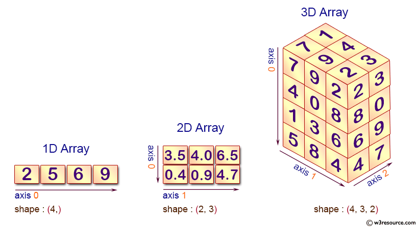
N-dimensional array (ndarray)
NumPy is used to work with arrays. The array
object in NumPy is called ndarray. We can
create a ndarray object by using the array()
function:
# Create an array from a list
arr = np.array([1, 2, 3, 4, 5, 6])

# Check the object
type(arr)

# Check the shape
np.shape(arr)
Every numpy array is a grid of elements of the
same type. Numpy provides a large set of
numeric datatypes that you can use to construct arrays.
Numpy tries to guess a datatype when you create an array,
but functions that construct arrays usually also include an optional
argument to explicitly specify the datatype. For example:
x = np.array([1, 2])
print(x.dtype)

y = np.array([1.0, 2.0])
print(y.dtype)

# Force a particular datatype
z = np.array([1, 2], dtype=np.int64)
print(z.dtype)
For more about numpy datatypes, check Data type objects.
You can also create arrays on various dimensions:
# 0-D
arr0 = np.array(1)
print(arr0)

# 1-D
arr1 = np.array([1, 2, 3, 4, 5, 6])
print(arr1)

# 2-D
arr2 = np.array([[1, 2, 3], [4, 5, 6]])
print(arr2)

# 3-D
arr3 = np.array([[[1, 2, 3], [4, 5, 6]], [[1, 2, 3], [4, 5, 6]]])
print(arr3)

# Use ndim to verify the dimensions
print(arr0.ndim)
print(arr1.ndim)
print(arr2.ndim)
print(arr3.ndim)
Reshaping
Reshaping means changing the shape of an array. The shape of an array is the number of elements in each dimension. By reshaping, we can add or remove dimensions or change number of elements in each dimension.
arr4 = np.array([1, 2, 3, 4, 5, 6, 7, 8, 9, 10, 11, 12])

# 1-D to 2-D
print(arr4.reshape(4, 3))

# 1-D to 3-D
print(arr4.reshape(2, 2, 3))

# This will return an error
print(arr4.reshape(2, 3, 4))

# This is fine, -1 means "unknown" dimension, python will compute it for you.
print(arr4.reshape(2, 3, -1))
Array creation
There are some built-in functions to create arrays, check the following lines:
# Create some uniform arrays
a1 = np.zeros((2,2))
print(a1)

a2 = np.full((3,3), np.pi)
print(a2)

a3 = np.ones_like(a1)
print(a3)

a4 = np.zeros_like(a2)
print(a4)
You can create an array in a defined range:
Indexing and slicing
Array indexing and slicing are the same as accessing a
list element. Remember, index starts from
0:
One thing new is integer array indexing:
# Make up an array
a = np.linspace(1,12,12).reshape(3,4)
print(a)

# integer array indexing: [0,2] and [1,0]
print(a[[0, 1], [2, 0]])

# integer array indexing: [0,2], [1,0], [-1,-1], and [2,2]
print(a[[0, 1, -1, 2], [2, 0, -1, 2]])

# one step more, change the array
# can you figure out why
b = [0, 1, 2]
print(a)
a[np.arange(3), b] += 100
print(a)
You can also use boolean indexing:
Array operations: basic math
Basic mathematical functions operate elementwise on arrays, and are available both as operator overloads and as functions in the numpy module:
# Make up two arrays
x = np.array([[1,2],[3,4]], dtype=np.float64)
y = np.array([[5,6],[7,8]], dtype=np.float64)

# Elementwise operator; both produce the array
print(x + y)
print(np.add(x, y))

# Difference
print(x - y)
print(np.subtract(x, y))

# Product
print(x * y)
print(np.multiply(x, y))

# Division
print(x / y)
print(np.divide(x, y))

# Square root
print(np.sqrt(x))
Please check Mathematical
functions for a list of all available functions in
numpy.
Array operations: matrix
Numpy uses the dot function to compute
inner products of vectors, to multiply a vector by a matrix, and to
multiply matrices. dot is available both as a function in
the numpy module and as an instance method of array
objects. For example:
# Make up two arrays
x1 = np.array([[1,2],[3,4]])
x2 = np.array([[5,6],[7,8]])

# Make up two more arrays
y1 = np.array([9,10])
y2 = np.array([11, 12])

# Inner product of vectors
print(y1.dot(y2))
print(np.dot(y1, y2))

# Matrix product
print(x1.dot(y1))
print(np.dot(x1, y1))

# Matrix product
print(x1.dot(x2))
print(np.dot(x1, x2))
To transpose a matrix, simply use the T attribute of an
array object:
Array operations: statistics
Numpy also provides a range of functions to compute
statistics of an array. For example:
x = np.linspace(1,12,12).reshape(4,3)

# Get the sum
np.sum(x)

# Get the sum along an axis, make sure you understand
np.sum(x, axis=0)
np.sum(x, axis=1)

# Get the max and min along an axis
np.amax(x)
np.amax(x, axis=0)
This figure shows the concept of “axis”
Please check Statistics
functions for a list of all available functions in
numpy.
Broadcasting
The term broadcasting describes how numpy
treats arrays with different shapes during arithmetic operations.
Subject to certain constraints, the smaller array is “broadcast” across
the larger array so that they have compatible shapes. Broadcasting
usually leads to efficient algorithm implementations.
When operating on two arrays, NumPy compares their
shapes element-wise. It starts with the trailing (i.e. rightmost)
dimensions and works its way left. Two dimensions are compatible
when:
they are equal, or
one of them is
1
If these conditions are not met, a
ValueError: operands could not be broadcast together
exception is thrown, indicating that the arrays have incompatible
shapes. The size of the resulting array is the size that is not
1 along each axis of the inputs.
# 4*3 array
x = np.array([[0,0,0], [10,10,10], [20,20,20], [30,30,30]])
print(x)

# 1*3 array
v = np.array([0, 1, 2])
print(v)

# 4*3 and 1*3 is compatible
# Add v to each row of x using broadcasting
y = x + v
print(y)

# 3*1 and 1*3 is compatible
x = x[:,0]
x = x[:, np.newaxis]
print(x)
v = np.array([0, 1, 2])
print(v)
y = x + v  # Add v to each row of x using broadcasting
print(y)
Please check this for more about broadcasting.
Joining Array
Joining means putting the contents of two or more arrays in a single
array. NumPy joins arrays by axes - we pass a sequence of
arrays that we want to join to the concatenate() function,
along with the axis. If the axis is not explicitly passed, it is taken
as 0. For example:
# Joining 1-D arrays
arr1 = np.array([1, 2, 3])
arr2 = np.array([4, 5, 6])
arr = np.concatenate((arr1, arr2))
print(arr)

# Joining 2-D arrays
arr1 = np.array([[1, 2], [3, 4]])
arr2 = np.array([[5, 6], [7, 8]])
arr = np.concatenate((arr1, arr2), axis=1)
print(arr)
Similar to concatenate(), hstack(),
vstack(), and dstack() can also join arrays.
Try those for yourself.
In-class exercises
Exercise #1
Create an array as follows:
Exercise #2
Generate a 1-D array of 10 random integers. Each integer
should be a number between 30 and 40
(inclusive).
[Hint: use np.random.randint() ]
Exercise #3
Create an array 1,2,3,np.nan,5,6,7,np.nan, replace all
nan values with -9999.
[Hint: use isnan() ]
Exercise #4
Create an array with np.random.uniform(1,50,20) (make
sure you understand it), then replace all values greater than
30 to 30 and less than 10 to
10.
[Hint: try np.where() function]
Exercise #5
Create an array with np.arange(20), replace all odd
numbers in the array with -1.
Exercise #6
Create two arrays (x and y) with
np.random.randint(), find elements in x where
its value is larger than its corresponding element in
y.
[Hint: try np.where() function]
Further reading
- Data Science Cheat SheetNumPy
- Python Numpy Array Tutorial
- Numpy official manual
- 100 numpy exercises (need VPN)
- Learn numpy (with a lot of resources)